Excel Power Query & P6 go hand-in-hand. Around two years ago, I realized that although my role as a project planner was based on my skills in Primavera P6, I was spending a significant amount of my day doing repetitive work in Excel. I would update my project schedules in P6 and then spend hours getting all the reports ready.
All this changed when I came across Excel’s new data transformation tool Power Query. Power Query came out as a plug-in for Excel 2014 and is now standard in all post 2014 excel products. Power Query is designed to transform and shape data into a format that can be organized though a pivot table. The reason this technique is so good for Primavera P6 users is that Primavera P6 is a database system and produces data that is formatted for Power Query.
The purpose of this tutorial is to show how the Primavera P6 report generating feature along with Power Query can allow you to quickly and accurately export complex data out of Primavera P6 and create understandable reports for other project members. I have found this feature very valuable in giving the project team a better understanding of the project plan and creating more confidence my role as a project planner.
This tutorial explains how to use Power Query for the following scenario: You have been asked to export the resource loading data from P6 into Excel to allow a project manager to investigate the resource usage of each work group over time. You are expecting a lot of changes to the schedule and resource curves due to the project deadlines and resource constraints. How do you export the data quickly and accurately to Excel every time you get project feedback?
Before you do this tutorial, please make sure that your version of Excel is more recent than 2014 and has a Data tab available in the ribbon at the top.
The tutorial is broken into three parts.
- How to export the resource assignments out of Primavera P6 into a CSV file using the report generating function.
- How to use Power Query in Excel to format the CSV file into a format that can be used in a Pivot Table / Pivot Chart.
- How to format the data into a report that a project manager can easily understand.
Part One – Exporting a CSV file from P6
Plan Academy has covered many ways to export P6 data to Excel, but this technique is a bit different. The first step is to set up the report generating option within Primavera P6 to generate a CSV file that contains the budgeted and budgeted cumulative hours spread over a month interval. This data will be in the same data format that you see when you click the resource assignment screen within Primavera P6.

Step 1
Add a new report to the Report section of Primavera P6.

Step 2
Using the report generating wizard, make sure to click the Time Distribution Data check mark, then click the Activity Resource and Role Assignments item.

Step 3
The next screen allows you to set the Columns, Group and Sort, and Filters that you want applied to the report. For this simple report example, we will only set the Columns option. Select and add Resource Name as the only column in the report.

Step 4
The next screen allows you to set the data that you want to see in the time distributed report. Click on Time Interval Fields and select Cum Budgeted Units and Budgeted Units.

Step 5
On the Timescale option, set the Date Interval to Month.

Step 6
Click Run Report. To select the format that the report will be exported in, select the ASCII Text File option and just use the default options that P6 uses. Set the location for the text file that P6 will export under Output file.

Step 7
Click Finish, and you now have a saved report that can be run against any project in Primavera P6.
Part Two – Importing a CSV File into Excel Using Power Query
The next step is to take the CSV file and convert it into a table format that can be analyzed using a Pivot Table or Pivot Chart. The big advantage to this technique is that in the future, when you export the CSV file again, you can simply refresh the excel workbook and the data will be updated.
Step 1
The first step is to go to the Data tab in excel and click on the Get Data option.

Step 2
Click From Text/CSV. You will have to go to the folder that you exported the CSV file into from P6.
Power Query will preview the CSV file and parse it into a table format. Now open Power Query and use the interface to shape the data into a format that you can use. Click Edit in order to do this.

Step 3
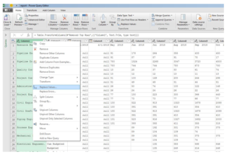
This is the Power Query interface. The transformations that you will add are listed on the right-hand side of the screen.
The first transformation that you want to perform is in Column 1. The resource names apply to both the Cum Budgeted row and the Budgeted row. The Primavera P6 export, however, skips the second row. You need to correct this and display the resource name in both rows.

Step 4
Depending on your version of Excel, Power Query may handle the data differently. You want the Date row to be in the first row of the table so that you can promote them as Table Headers later on.
If your table has the dates in row 1, do nothing and skip to Step 5.
If row 1 contains empty cells, follow the next step to remove the empty row and position the date rows in the correct place.
Click on the Remove Top Rows option, enter 1 into the pop-up box and click OK.

Step 5
Now you need to correct the data in Column 1. First, you want to remove any spaces around the text in Column 1 by using the Trim feature. To do this, right click on Column 1, go to Transform and then click Trim.

Step 6
There is still a problem. You want the blank spaces in Column 1 to contain null for the next step. To do this, right click on Column 1 and select Replace Values…

Step 7
In the pop-up box, leave the Value to Find box blank as that represents the empty spaces. In the Replace With box type in null and click OK.
The blank cells in Column 1 now contain null.

Step 8
Now right click on Column 1 and select Fill and then Down. Now the Resource Names in Column 1 are correctly tagged to each row.

Step 9
The second transformation is to unpivot the time distributed data into two columns; one column to contain the dates and another column to contain the hour data.
Technically you are normalizing the data. Primavera P6 displays the data in a way that is easy for humans to read and understand. You want to undo this step and create a very long table that can be used by the Pivot Table and Pivot Chart features in Excel. Both pivoting and unpivoting data are very useful features in Power Query.
You want to use the data in Row 1 as the column headers on the table. Double check that the monthly dates for the resource distribution are in Row 1. Then click the Use First Row as Headers option on the Toolbar, as shown below.

Step 10
The header title on Column 2 is not what you want. Rename it to Units by double clicking on the column header and typing in “Units”.

Step 11
Now for the unpivot step.
This is where you take the time distributed columns and rearrange that data into one single column that can be used in a pivot table.
You want to unpivot the date columns only – Columns 3, 4, 5, and onward. You want to preserve Columns 1 & 2. In the future, you may extend the schedule and add more date columns.
To allow the query to work in the future, you select the first two columns by holding Shift and selecting them. Then, right-click and choose Unpivot Other Columns.
This unpivots all the data columns for Budgeted Units and Cumulative Units into the format that you need.

Step 12
Click on the filter button in the Units column. Make sure that you only have Budgeted and Cum Budgeted text selected. If you have a Null or Blank text in this section, uncheck this option as you do not want to include those rows.

Step 13
The Date column has been renamed to “Attribute” and the data here is categorized as text.
You will want to change this to a Date-type field.
You also want the Date field to show correctly even if you email the file to another country where the end user has a different date format on their computer.
To do this, you click on the ABC-icon to the left of the column title and click Using Locale…

Step 14
In the drop-down menu, change Data Type to Date and Locale to English (United States). You will want to use whatever Locale is setup on your computer. Click OK.

Step 15
Now go to the Value column, click on the ABC123-icon to the left of the column title and select Decimal Number.

Step 16
The final step is to rename columns 3 (Attribute) and 4 (Value) to be Date and Hours. You do this by double clicking on the column header and typing the correct text.

Step 17
The query is now finished. The resource name issue has been fixed and the date and hours data are unpivoted.
Now you want to return the data to your excel worksheet as a table and use the table to create a Pivot Chart.
Click Close and Load To.. in the top left corner of the screen.

You want the data returned as a table in a new tab so select the following options.

Part 3 – Using The Data in a Pivot Chart
You have taken the CSV file from Primavera P6 and transformed it into a table that can be manipulated by a pivot table or pivot chart.
Step 1
Now let’s create the Pivot Table.
Highlight the entire table, click on the Insert tab and select Pivot Chart. In the option box, click New Worksheet.

In order to set up the Pivot Chart, drag the right columns into the appropriate Pivot Chart Fields.
Drag & drop the Date column into the Axis categories.
Drag & drop the Units into the Legend (Series).
Drag & drop the Hours column into the Values section.
When you dropped the Date column into the Axis(Categories) section, Excel automatically adds Years and Quarters to the date data. To get the chart to display in months, click on the plus symbol in the bottom right corner of the chart until you see months on the x-axis.
The Pivot Chart now contains the Budgeted Units and Cumulative Budgeted Units for the project. You need to convert the Cumulative Budgeted Units into a Line and assign it a secondary axis.

In order to format the CUM Budgeted properly, click on the chart and select Change Chart Type.

Select the Combo option on the left side of the Change Chart Type menu. The Budgeted series should be a Clustered Column and be on the Primary Axis (secondary axis is not selected). The Cum Budgeted series should be a Line and the Secondary Axis box should be checked. This will display the budgeted units as column with the quantity on the left-hand side and the Cum Budgeted units as a line with the quantity on the right-hand side.

You’re almost done. You want to give the project manager the ability to click on each engineering discipline and see the Budgeted Units for each discipline over time. This will allow them to review the plan in detail with their team. Luckily, as you are working with a pivot chart, this is no big deal. Go to the PivotChart Fields section and right click on the Resource Name line and select Add as Slicer.

The Primavera P6 data has been converted into a Pivot Chart format and the project manager can go through each discipline and review the Budgeted Units. If there are last-minute changes (there usually are), you simply update Primavera P6 and export a new CSV file. All the project manager needs to do is refresh and the updated data will be imported and instantly usable.
The image below shows how the slicer can be used to select a resource or a group of resources. The hours per month and cumulative hours adjust to each selection, giving the project manager the ability to dig through the data.

The final step is to clean up the Cumulative Budgeted Line. When you exported the data from Primavera P6 the report included 4 months too much of cumulative data. Remove this by clicking on the Data tab, selecting Queries and Connections, opening the Query that was just created, and clicking on the drop-down menu at the top of the date column. Filter the dates to include dates that are before the 1st of February 2019. Then click Close and Load in the top left corner and the Pivot Chart will update and display the data correctly. You will have to adjust this filter in the future if the project schedule changes and the resources push past the 1st of February.


Finally, remember that once the query is set up and you update the CSV data source, you will have to update the link between Power Query and the source file. You do this by selecting Refresh All in the Data tab.

I hope that this tutorial gave you a useful introduction to what Power Query can do. I have found it to be a valuable tool that drastically helps reduce repetitive tasks and I hope that it can help you out too.
Let us know what you think by leaving a comment below.