Primavera users are also Excel users. As many of you know, Microsoft Excel has many useful functions in different areas such as Financial, Date & Time, Math & Trig and so on. One of these areas is Look up & Reference. The functions in this area are dealt with lists, indexes and arrays and help us to find some special information in these listed data or other. This required information could be address of a desired cell which contains some special value, a value or action to perform a list of values, a reference specified by a text string, a relative position of an item in array that matches a specified value in a specific order and finally: a value in the leftmost column of a table and then returns a value in the same row from a column you specify.
The last function is called VLOOKUP and I myself find it very useful in most of the planning activities. Sometimes when you have some spreadsheets with heaps of information in them and you need to transfer some updated information from one list into another, VLOOKUP helps you to do it fast and accurate. This list could be your export from Primavera and you can update it from a database (which most of the time can have an output in the form of a spreadsheet) using VLOOKUP and then import it in Primavera and everything is updated now, easy and quick! Let’s see how can we define and use this function in our Excel Vlookup tutorial.
How to write a VLOOKUP formula
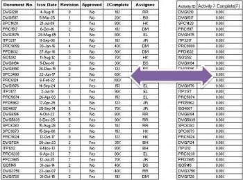
Let’s start with a practical example. Suppose that we have a list of updated progress of some documents and we want to update their percent completes in another list which has been exported from Primavera. Here are our lists:.

Let’s call the right table Database table and the left one Primavera table. Now we want to have percent complete for each document. So we start writing the formula in the Activity % complete column in primavera table.

When you choose VLOOKUP function in Excel, you should complete the following inputs:
- Lookup_value: This is the value that is common between our arrays and we use it to find our desired value. In this example both arrays have Documents numbers in common, so we use this value as our look up value.
- Table_array: In here we should input the address of our main array that have desired information in it and in which data is retrieved. We will see how we should insert the cell address in here.
- Col_index_num: This number is the column number in our main array in which our desired data is located. You should notice that this number starts from one for the first column in the array that you have chosen in the previous section, so you should count columns to find your result column and input the number in here. In our example %Complete is located in fifth column so we should input 5 in this part.
- Range_lookup: In this part you have two logical TRUE and FALSE options and each one have different meanings in the formula. If you put TRUE the function search for the closest match in the array and you should note that the search is in the ascending order. If you leave this section blank, it works like you put TRUE in it. FALSE means you need to find an exact match in the array, so this option is more accurate and reliable and I prefer this one because sometimes especially when you search some numbers , using TRUE makes you confused.
Now let’s get back to our example. The Lookup_value for our example is Activity IDs in the primavera table which is called Document Number in the database table. Our Table_array starts from the first column in the database table and ends on %complete column which is our desired column for getting the result. Col_index is the column number of %complete column which is 5. For getting the most accurate result let’s put the FALSE in the Range_lookup.
So our formula is like this:

As you can see for the Table_array amount, the address of cells in the array has been inserted completely, rows and columns, sheet name and even file name is identified. In Excel wherever you see $ sign it means that amount is fixed and if you drag the formula it is not going to be changed, so here the column and the row are both fixed and when you drag the formula for the rest of activities your array is the same but otherwise if you have not $ sign in there and you drag the formula the next one would starts from column C and row 2 till column F and row 32.
Now we can take a look at results and they are amazing. We have our updated list very easy and quick:

Tips
For using Vlookup function there are some tips that you should consider them:
- Always your lookup value should be in the first column of your table array. If you do not obey this rule the formula won’t work for you. In our example the formula searches the Document Number column to find out our Activity IDs and return their %complete and this column is the first one in the selected array. Sometimes you have to replace columns to put your look up value in the first place of the array.
- When your lookup value is a text instead of numbers the format of tables are important and you need to make them similar to each other, then the formula can find the result.
- After writing the formula and drag it for all the cells of the column, maybe the result would appear in another category. In our example if I haven’t set the category of percentage for Activity % complete column in primavera table, the data could be appeared in the decimal number format. Therefore, you need to be sure that you set the proper format for that column.
- You remember that in the table_array part of the formula when you choose the array by dragging on the cells,the complete address of the array apppears in the formula. On the other hand, most of the time your result is getting from a different file.Sometimes when you close and save both files and then change the place of the reference file (in our example database file) in your computer the formula gets confused and gives you errors. Consequently you may lose your results. I prefer to copy and paste the value of formula after checking that it has worked correctly. So it doesn’t matter where I’m going to save the reference file and the next time when I open the main file, the lookup values are on their place in the file and I have them.
Conclusion
Vlookup is one of the most useful functions in Excel especially for planners and it helps you to save your time and have many updated spreadsheet for either importing to primavera or preparing reports and charts by them. But you should consider the tips and always check the results randomly to be sure that the formula has worked correctly, because this function has many dependencies and if you miss to obey all the rules you may get the wrong results, but when you get used to it, there won’t be any error and you just enjoy its quickness.